Step 1-6

Load the R pacakeges we will use.

library(tidyverse)
library(echarts4r)

Read the data in the files drug_cos.csv , health_cos.csv in to R and assign to the variables drug_cos and health_cos, respectively

drug_cos  <- read_csv("https://estanny.com/static/week6/drug_cos.csv")
health_cos <- read_csv("https://estanny.com/static/week6/health_cos.csv")

Use glimpseto get a glimpse of the data

drug_cos %>% glimpse()

Rows: 104
Columns: 9
$ ticker       <chr> "ZTS", "ZTS", "ZTS", "ZTS", "ZTS", "ZTS", "ZTS"…
$ name         <chr> "Zoetis Inc", "Zoetis Inc", "Zoetis Inc", "Zoet…
$ location     <chr> "New Jersey; U.S.A", "New Jersey; U.S.A", "New …
$ ebitdamargin <dbl> 0.149, 0.217, 0.222, 0.238, 0.182, 0.335, 0.366…
$ grossmargin  <dbl> 0.610, 0.640, 0.634, 0.641, 0.635, 0.659, 0.666…
$ netmargin    <dbl> 0.058, 0.101, 0.111, 0.122, 0.071, 0.168, 0.163…
$ ros          <dbl> 0.101, 0.171, 0.176, 0.195, 0.140, 0.286, 0.321…
$ roe          <dbl> 0.069, 0.113, 0.612, 0.465, 0.285, 0.587, 0.488…
$ year         <dbl> 2011, 2012, 2013, 2014, 2015, 2016, 2017, 2018,…

health_cos %>% glimpse()

Rows: 464
Columns: 11
$ ticker      <chr> "ZTS", "ZTS", "ZTS", "ZTS", "ZTS", "ZTS", "ZTS",…
$ name        <chr> "Zoetis Inc", "Zoetis Inc", "Zoetis Inc", "Zoeti…
$ revenue     <dbl> 4233000000, 4336000000, 4561000000, 4785000000, …
$ gp          <dbl> 2581000000, 2773000000, 2892000000, 3068000000, …
$ rnd         <dbl> 427000000, 409000000, 399000000, 396000000, 3640…
$ netincome   <dbl> 245000000, 436000000, 504000000, 583000000, 3390…
$ assets      <dbl> 5711000000, 6262000000, 6558000000, 6588000000, …
$ liabilities <dbl> 1975000000, 2221000000, 5596000000, 5251000000, …
$ marketcap   <dbl> NA, NA, 16345223371, 21572007994, 23860348635, 2…
$ year        <dbl> 2011, 2012, 2013, 2014, 2015, 2016, 2017, 2018, …
$ industry    <chr> "Drug Manufacturers - Specialty & Generic", "Dru…

Which variables are the same in both data sets

names_drug <-drug_cos %>%  names()
names_health <-health_cos %>%  names()
intersect(names_drug, names_health)

[1] "ticker" "name"   "year"

Select subset of variables to work with

For drug_cos select (in this order): ticker, year, grossmargin
Extract observations for 2018
Assign output to drug_subset
For health_cos select (in this order): ticker, year, revenue, gp , industry
Extract observations for 2018
Assign output to health_subset

drug_subset  <-drug_cos %>% 
select(ticker, year, grossmargin) %>% 
  filter(year == 2018)

Keep all the rows and column drug_subset join with column in health_subset

drug_subset %>% left_join(drug_subset)

# A tibble: 13 × 3
   ticker  year grossmargin
   <chr>  <dbl>       <dbl>
 1 ZTS     2018       0.672
 2 PRGO    2018       0.387
 3 PFE     2018       0.79 
 4 MYL     2018       0.35 
 5 MRK     2018       0.681
 6 LLY     2018       0.738
 7 JNJ     2018       0.668
 8 GILD    2018       0.781
 9 BMY     2018       0.71 
10 BIIB    2018       0.865
11 AMGN    2018       0.827
12 AGN     2018       0.861
13 ABBV    2018       0.764

Question join_ticker

Start with the drug_cos data

Extract observations for the ticker **** from drug_cos Assign output to the variabledrug_cos_subset`

drug_cos_subset <- drug_cos %>% 
  filter(ticker == "JNJ")

combo_df <- drug_cos_subset %>% 
  left_join(health_cos)

display drug_cos_subset

drug_cos_subset

# A tibble: 8 × 9
  ticker name  location ebitdamargin grossmargin netmargin   ros   roe
  <chr>  <chr> <chr>           <dbl>       <dbl>     <dbl> <dbl> <dbl>
1 JNJ    John… New Jer…        0.247       0.687     0.149 0.199 0.161
2 JNJ    John… New Jer…        0.272       0.678     0.161 0.218 0.173
3 JNJ    John… New Jer…        0.281       0.687     0.194 0.224 0.197
4 JNJ    John… New Jer…        0.336       0.694     0.22  0.284 0.217
5 JNJ    John… New Jer…        0.335       0.693     0.22  0.282 0.219
6 JNJ    John… New Jer…        0.338       0.697     0.23  0.286 0.229
7 JNJ    John… New Jer…        0.317       0.667     0.017 0.243 0.019
8 JNJ    John… New Jer…        0.318       0.668     0.188 0.233 0.244
# … with 1 more variable: year <dbl>

display combo_df

combo_df

# A tibble: 8 × 17
  ticker name  location ebitdamargin grossmargin netmargin   ros   roe
  <chr>  <chr> <chr>           <dbl>       <dbl>     <dbl> <dbl> <dbl>
1 JNJ    John… New Jer…        0.247       0.687     0.149 0.199 0.161
2 JNJ    John… New Jer…        0.272       0.678     0.161 0.218 0.173
3 JNJ    John… New Jer…        0.281       0.687     0.194 0.224 0.197
4 JNJ    John… New Jer…        0.336       0.694     0.22  0.284 0.217
5 JNJ    John… New Jer…        0.335       0.693     0.22  0.282 0.219
6 JNJ    John… New Jer…        0.338       0.697     0.23  0.286 0.229
7 JNJ    John… New Jer…        0.317       0.667     0.017 0.243 0.019
8 JNJ    John… New Jer…        0.318       0.668     0.188 0.233 0.244
# … with 9 more variables: year <dbl>, revenue <dbl>, gp <dbl>,
#   rnd <dbl>, netincome <dbl>, assets <dbl>, liabilities <dbl>,
#   marketcap <dbl>, industry <chr>

Assign the company location to co_name

co_name <- combo_df %>% 
  distinct(name) %>% 
  pull ()

Assign the company location to co_location

co_location <- combo_df %>% 
  distinct(location) %>% 
  pull ()

combo_df_subset  <- combo_df  %>% 
  select( year,  grossmargin,  netmargin, 
   revenue,  gp,  netincome)

Assign the company’s industry group to the variabl co_industry

co_industry <-combo_df %>% 
  select(industry) %>% 
  pull()

Start with health_cos
Extract observations for the ILMN ticker from health_cos
Assign output to the variable health_cos_subset

health_cos_subset <- health_cos %>% 
  filter(ticker == "ILMN")

Create the variable grossmargin_check to compute with the variable grossmargin they should be equal. grossmargin_check = gp / revenue

Create the variable close_enough to check that the absolute value of the difference between grossmargin_check and grossmargin is less than .001

combo_df_subset %>% 
  mutate(grossmargin_check = gp / revenue, 
         close_enough = abs(grossmargin_check - grossmargin) <0.001)

# A tibble: 8 × 8
   year grossmargin netmargin     revenue          gp   netincome
  <dbl>       <dbl>     <dbl>       <dbl>       <dbl>       <dbl>
1  2011       0.687     0.149 65030000000 44670000000  9672000000
2  2012       0.678     0.161 67224000000 45566000000 10853000000
3  2013       0.687     0.194 71312000000 48970000000 13831000000
4  2014       0.694     0.22  74331000000 51585000000 16323000000
5  2015       0.693     0.22  70074000000 48538000000 15409000000
6  2016       0.697     0.23  71890000000 50101000000 16540000000
7  2017       0.667     0.017 76450000000 51011000000  1300000000
8  2018       0.668     0.188 81581000000 54490000000 15297000000
# … with 2 more variables: grossmargin_check <dbl>,
#   close_enough <lgl>

Create the variable margin_check to compare with the variable netmargin they should be equal.

Create the variable close_enough to check that the absolute value of the difference between netmargin_check and netmargin is less than 0.001

combo_df_subset %>% 
  mutate(netmargin_check = netincome / revenue, 
         close_enough = abs(netmargin_check - netmargin) < 0.001)

# A tibble: 8 × 8
   year grossmargin netmargin     revenue          gp   netincome
  <dbl>       <dbl>     <dbl>       <dbl>       <dbl>       <dbl>
1  2011       0.687     0.149 65030000000 44670000000  9672000000
2  2012       0.678     0.161 67224000000 45566000000 10853000000
3  2013       0.687     0.194 71312000000 48970000000 13831000000
4  2014       0.694     0.22  74331000000 51585000000 16323000000
5  2015       0.693     0.22  70074000000 48538000000 15409000000
6  2016       0.697     0.23  71890000000 50101000000 16540000000
7  2017       0.667     0.017 76450000000 51011000000  1300000000
8  2018       0.668     0.188 81581000000 54490000000 15297000000
# … with 2 more variables: netmargin_check <dbl>, close_enough <lgl>

Question Summarize_industry

Use health_cos

health_cos %>% 
  group_by(industry) %>% 
  summarize(mean_netmargin_perecent = mean( netincome / revenue) *100 , 
  median_netmargin_perecent = median( netincome / revenue) *100 , 
  min_netmargin_perecent = min( netincome / revenue) *100,
  max_netmargin_perecent = max( netincome / revenue) *100)

# A tibble: 9 × 5
  industry          mean_netmargin_… median_netmargi… min_netmargin_p…
  <chr>                        <dbl>            <dbl>            <dbl>
1 Biotechnology                -4.66             7.62         -197.   
2 Diagnostics & Re…            13.1             12.3             0.399
3 Drug Manufacture…            19.4             19.5           -34.9  
4 Drug Manufacture…             5.88             9.01          -76.0  
5 Healthcare Plans              3.28             3.37           -0.305
6 Medical Care Fac…             6.10             6.46            1.40 
7 Medical Devices              12.4             14.3           -56.1  
8 Medical Distribu…             1.70             1.03           -0.102
9 Medical Instrume…            12.3             14.0           -47.1  
# … with 1 more variable: max_netmargin_perecent <dbl>

mean_netmargin_percent for the industry Medical Care Facilities is 6.10% median_netmargin_percent for the industry Medical Care Facilities is 6.10% min_netmargin_percent for the industry Biotechnology is -4.65% max_netmargin_percent for the industry Diagnostics & Research is 13.13%

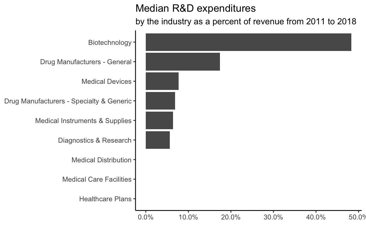
Prepare the data for the plots

Start with health_cos THEN group_by industry THEN calculate the median research and development expenditure by industry assign the output to df

df <- health_cos %>% 
  group_by(industry) %>% 
  summarize(med_rnd_rev = median(rnd/revenue))

Use glimpse to glimps the data for the plots

df %>% glimpse()

Rows: 9
Columns: 2
$ industry    <chr> "Biotechnology", "Diagnostics & Research", "Drug…
$ med_rnd_rev <dbl> 0.48317287, 0.05620271, 0.17451442, 0.06851879, …

Create a static bar chart

use ggplot to initialize the chart data is df the variable industry is mapped to the x-axis - reoder it based the value of med_rnd_rev the variable med_rnd_rev is mapped to the y-axis add a bar chart using geom_col use scale_y_continous to label the y-axis with percent use coord_flip() to flip the coordinates use labs to add tittle, subtitle and remove x and y-axes use theme_ipsum() from the hrbrthemes pacakges to improve the theme

ggplot(data = df, 
   mapping = aes( 
       x = reorder(industry, med_rnd_rev) ,
       y = med_rnd_rev
       )) +
  geom_col()+
  scale_y_continuous(labels = scales::percent) +
  coord_flip() +
  labs(
    title = "Median R&D expenditures" , 
    subtitle = "by the industry as a percent of revenue from 2011 to 2018",
    x = NULL , y = NULL) +
theme_classic()

Save the last plot to previewpng and add to the yaml chunk at the top.

{r}save(filename= "preview.png" , path = here::here("_posts", "2001-02-27-joining data")) 11. Create an interative bar chart using the package [echarts4r] (https://echarts4r.john-coene.com/index.html)

start with the data df use arrange to reorder med_rnd_rev use e_charts to initialize a chart the variable industry is mapped to the x-axis add a bar chart using e_bar with the values of med_rnd_rev use e_flip_coords() to flip the coordinates use e_title to add the title and the subtitle use e_legend remove the legends use e_x_axis to change the format of the labels on the x-axis to percent use e_y_axis to remove the labels from the y-axis use e_theme to change the theme. find more themes here

df %>% 
arrange(med_rnd_rev) %>% 
e_charts( x = industry
   ) %>% 
e_bar(
  serie = med_rnd_rev,  
  name = "median"
  ) %>% 
e_flip_coords() %>% 
e_tooltip() %>% 
e_title(
  text = "Median industry R&D expenditures" ,
  subtext = "by industry as a percent of revenue from 2011 to 2018" ,
  left = "center") %>% 
e_legend(FALSE) %>% 
e_x_axis(
  formatter = e_axis_formatter("percent", digits = 0)
) %>% 
e_y_axis(
 show = FALSE
) %>% 
  e_theme("infographic")

Joining Data

Step 1-6

Question join_ticker

Question Summarize_industry