Sampling

A short description of the post.

library(tidyverse)
library(moderndive)

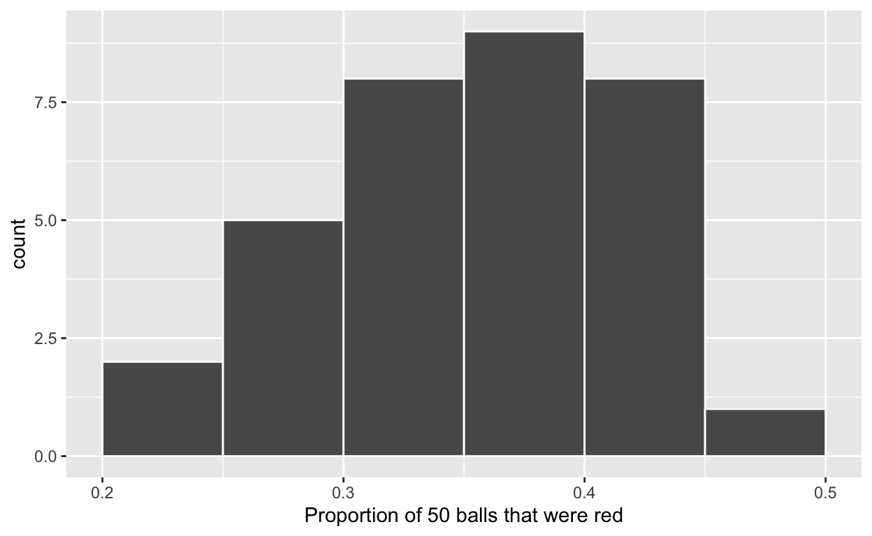
ggplot(tactile_prop_red, aes(x = prop_red)) + 
  geom_histogram(binwidth = 0.05, boundary = 0.4, color = "white") +
  labs(x = "Proportion of 50 balls that were red", 
       tittle = "Distribution of 33 proportions red")

set.seed(678)
virtual_shovel  <- bowl %>% 
  rep_sample_n(size = 50, reps = 1)
virtual_shovel

# A tibble: 50 × 3
# Groups:   replicate [1]
   replicate ball_ID color
       <int>   <int> <chr>
 1         1    2105 red  
 2         1     796 white
 3         1     681 red  
 4         1     920 red  
 5         1    1019 white
 6         1     653 white
 7         1    1295 white
 8         1    1736 white
 9         1    1450 red  
10         1    2009 red  
# … with 40 more rows

virtual_shovel %>% 
  mutate(is_red = (color == "red")) %>% 
  summarize(num_red = sum(is_red))  %>% 
  mutate(prop_red = num_red / 50)

# A tibble: 1 × 3
  replicate num_red prop_red
      <int>   <int>    <dbl>
1         1      19     0.38

virtual_shovel %>% 
  summarize(num_red = sum(color == "red")) %>% 
  mutate(prop_red = num_red / 50)

# A tibble: 1 × 3
  replicate num_red prop_red
      <int>   <int>    <dbl>
1         1      19     0.38

virtual_samples  <- bowl %>% 
  rep_sample_n(size = 50, reps = 33)
virtual_samples

# A tibble: 1,650 × 3
# Groups:   replicate [33]
   replicate ball_ID color
       <int>   <int> <chr>
 1         1    1770 red  
 2         1     971 red  
 3         1    1882 white
 4         1    2145 white
 5         1    1753 red  
 6         1     449 white
 7         1     943 white
 8         1     490 white
 9         1     401 white
10         1    2008 white
# … with 1,640 more rows

virtual_samples %>% 
  count(replicate)

# A tibble: 33 × 2
# Groups:   replicate [33]
   replicate     n
       <int> <int>
 1         1    50
 2         2    50
 3         3    50
 4         4    50
 5         5    50
 6         6    50
 7         7    50
 8         8    50
 9         9    50
10        10    50
# … with 23 more rows

virtual_samples %>% 
  group_by(replicate) %>% 
  count(color)

# A tibble: 66 × 3
# Groups:   replicate [33]
   replicate color     n
       <int> <chr> <int>
 1         1 red      16
 2         1 white    34
 3         2 red      17
 4         2 white    33
 5         3 red      22
 6         3 white    28
 7         4 red      22
 8         4 white    28
 9         5 red      18
10         5 white    32
# … with 56 more rows

virtual_prop_red  <- virtual_samples %>% 
  group_by(replicate) %>% 
  summarize(red = sum(color == "red")) %>% 
  mutate(prop_red = red / 50)
virtual_prop_red

# A tibble: 33 × 3
   replicate   red prop_red
       <int> <int>    <dbl>
 1         1    16     0.32
 2         2    17     0.34
 3         3    22     0.44
 4         4    22     0.44
 5         5    18     0.36
 6         6    22     0.44
 7         7    18     0.36
 8         8    20     0.4 
 9         9    23     0.46
10        10    19     0.38
# … with 23 more rows

virtual_samples_25  <- bowl %>% 
  rep_sample_n(size = 25, reps = 1000)

virtual_prop_red_25  <- virtual_samples_25 %>% 
  group_by(replicate) %>% 
  summarize(red = sum(color =="red")) %>% 
  mutate(prop_red = red / 25)

ggplot(virtual_prop_red_25, aes(x = prop_red)) +
  geom_histogram(binwidth = 0.05, boundary = 0.4, color = "white")

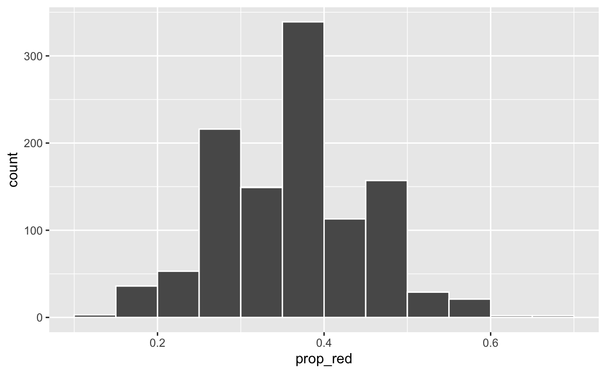
labs(x= "proportion of 25 balls that were red",
     title = "Distribution of 1000 proportions red")

$x
[1] "proportion of 25 balls that were red"

$title
[1] "Distribution of 1000 proportions red"

attr(,"class")
[1] "labels"

virtual_samples_50  <- bowl %>% 
  rep_sample_n(size = 50, reps = 1000)

virtual_prop_red_50  <- virtual_samples_50 %>% 
  group_by(replicate) %>% 
  summarize(red = sum(color =="red")) %>% 
  mutate(prop_red = red / 50)

ggplot(virtual_prop_red_50, aes(x = prop_red)) +
  geom_histogram(binwidth = 0.05, boundary = 0.4, color = "white")

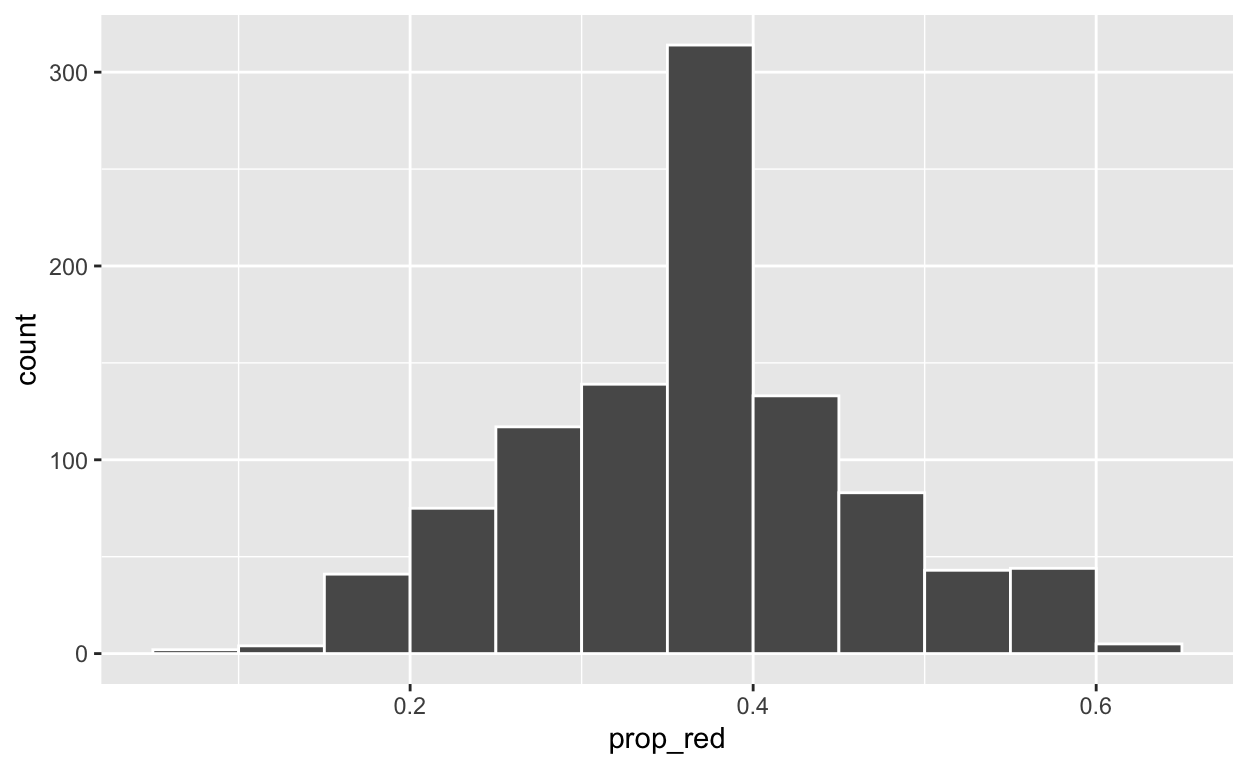
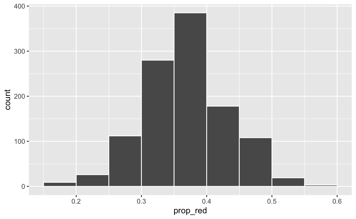
labs(x= "proportion of 50 balls that were red", 
     title = "Distribution of 1000 proportions red")

$x
[1] "proportion of 50 balls that were red"

$title
[1] "Distribution of 1000 proportions red"

attr(,"class")
[1] "labels"

virtual_samples_100  <- bowl %>% 
  rep_sample_n(size = 100, reps = 1000)

virtual_prop_red_100  <- virtual_samples_100 %>% 
  group_by(replicate) %>% 
  summarize(red = sum(color =="red")) %>% 
  mutate(prop_red = red / 50)

ggplot(virtual_prop_red_100, aes(x = prop_red)) +
  geom_histogram(binwidth = 0.05, boundary = 0.4, color = "white")

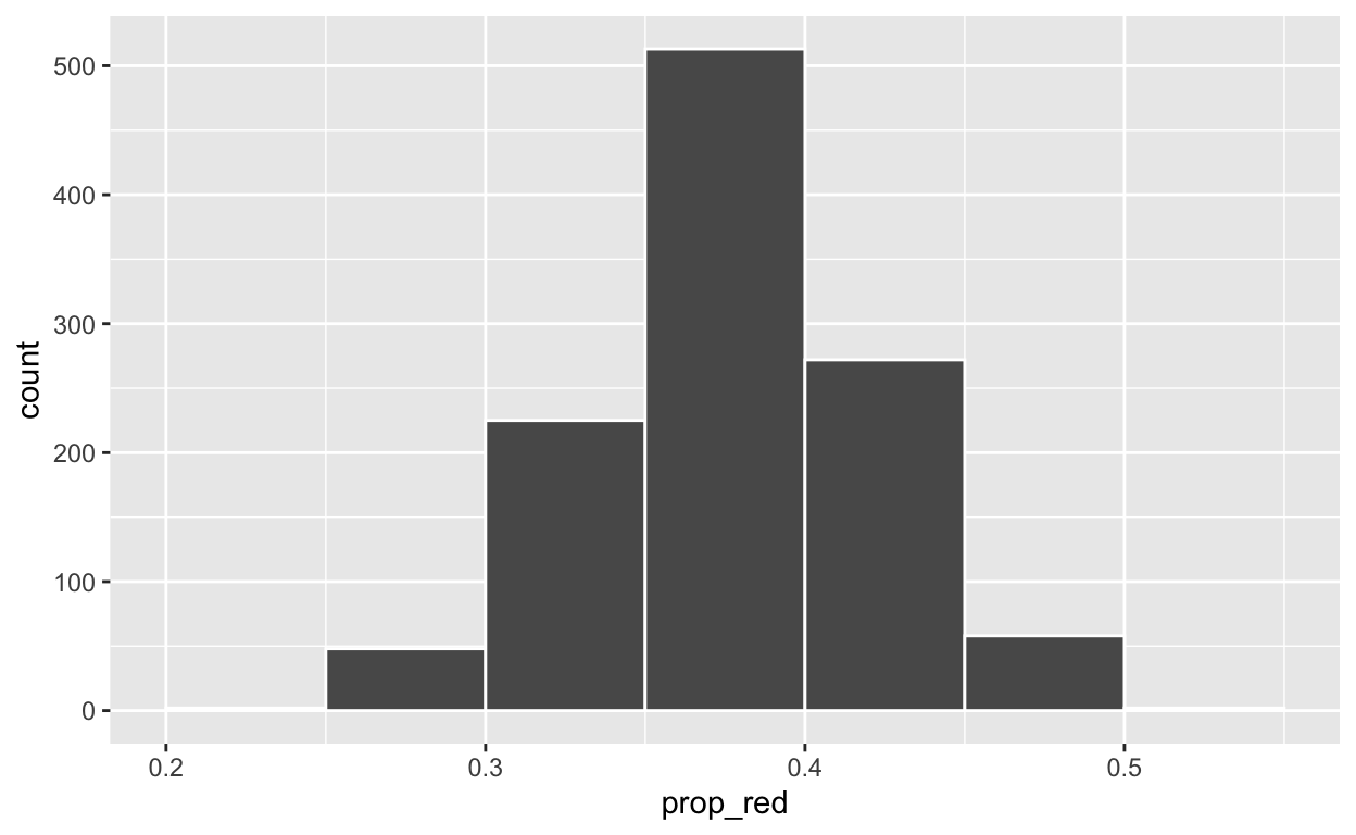
labs(x= "proportion of 100 balls that were red", 
     title = "Distribution of 1000 proportions red")

$x
[1] "proportion of 100 balls that were red"

$title
[1] "Distribution of 1000 proportions red"

attr(,"class")
[1] "labels"

virtual_prop_red_25 %>% 
  summarize(sd= sd(prop_red))

# A tibble: 1 × 1
      sd
   <dbl>
1 0.0967

virtual_prop_red_50 %>% 
  summarize(sd= sd(prop_red))

# A tibble: 1 × 1
      sd
   <dbl>
1 0.0677

virtual_prop_red_100 %>% 
  summarize(sd= sd(prop_red))

# A tibble: 1 × 1
      sd
   <dbl>
1 0.0941

virtual_samples_30  <- bowl %>% 
  rep_sample_n(size = 30, reps = 1120)

virtual_prop_red_30  <- virtual_samples_30 %>% 
  group_by(replicate) %>% 
  summarize(red = sum(color =="red")) %>% 
  mutate(prop_red = red / 30)

ggplot(virtual_prop_red_30, aes(x = prop_red)) +
  geom_histogram(binwidth = 0.05, boundary = 0.4, color = "white")

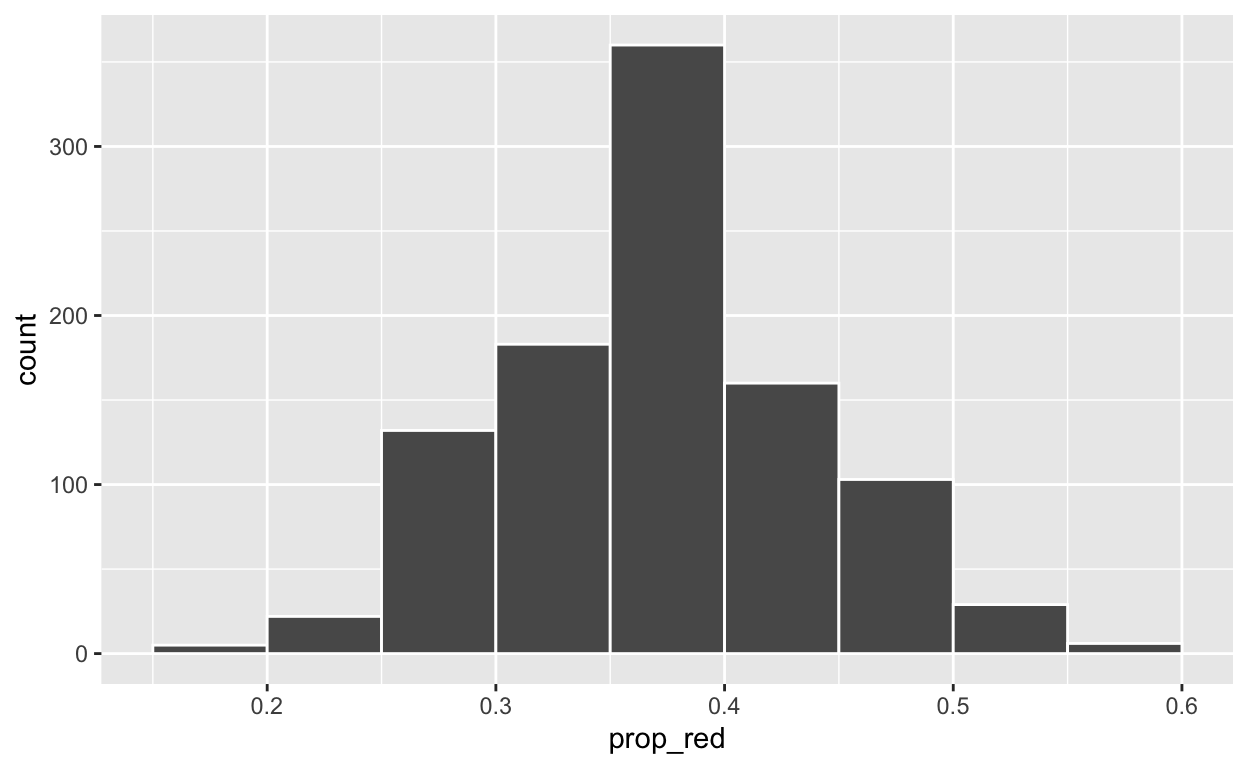
labs(x= "proportion of 30 balls that were red", 
     title = "Distribution of 1120 proportions red")

$x
[1] "proportion of 30 balls that were red"

$title
[1] "Distribution of 1120 proportions red"

attr(,"class")
[1] "labels"

virtual_samples_55  <- bowl %>% 
  rep_sample_n(size = 55, reps = 1120)

virtual_prop_red_55  <- virtual_samples_55 %>% 
  group_by(replicate) %>% 
  summarize(red = sum(color =="red")) %>% 
  mutate(prop_red = red / 55)

ggplot(virtual_prop_red_55, aes(x = prop_red)) +
  geom_histogram(binwidth = 0.05, boundary = 0.4, color = "white")

labs(x= "proportion of 55 balls that were red", 
     title = "Distribution of 1120 proportions red")

$x
[1] "proportion of 55 balls that were red"

$title
[1] "Distribution of 1120 proportions red"

attr(,"class")
[1] "labels"

virtual_samples_114  <- bowl %>% 
  rep_sample_n(size = 114, reps = 1120)

virtual_prop_red_114  <- virtual_samples_114 %>% 
  group_by(replicate) %>% 
  summarize(red = sum(color =="red")) %>% 
  mutate(prop_red = red / 114)

ggplot(virtual_prop_red_114, aes(x = prop_red)) +
  geom_histogram(binwidth = 0.05, boundary = 0.4, color = "white")

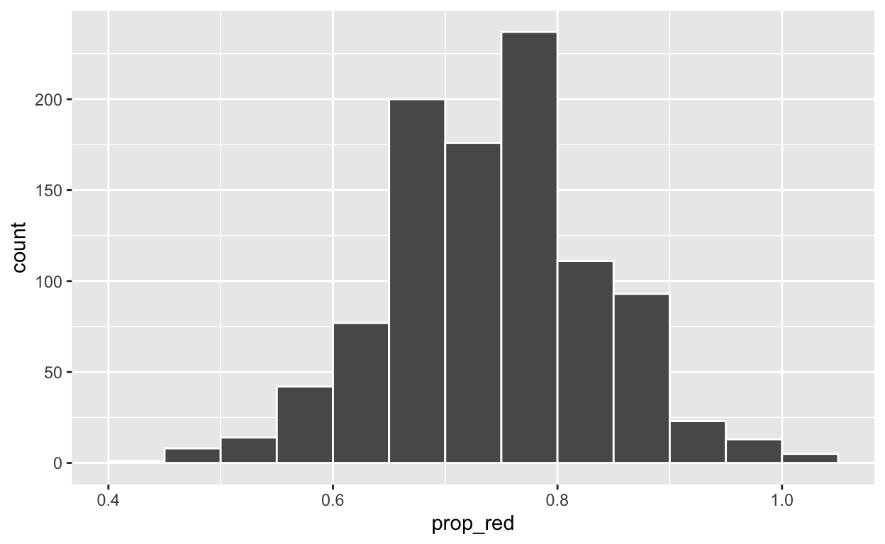
labs(x= "proportion of 114 balls that were red", 
     title = "Distribution of 1120 proportions red")

$x
[1] "proportion of 114 balls that were red"

$title
[1] "Distribution of 1120 proportions red"

attr(,"class")
[1] "labels"

virtual_prop_red_30 %>% 
  summarize(sd= sd(prop_red))

# A tibble: 1 × 1
      sd
   <dbl>
1 0.0872

virtual_prop_red_55 %>% 
  summarize(sd= sd(prop_red))

# A tibble: 1 × 1
      sd
   <dbl>
1 0.0639

virtual_prop_red_114 %>% 
  summarize(sd= sd(prop_red))

# A tibble: 1 × 1
      sd
   <dbl>
1 0.0449